Yield Memory - A Novel Concept to Assess Yield Variability

Something went wrong. Please try again later...

Crop Insights written by Rai A. Schwalbert and Ignacio A. Ciampitti, Ph.D., Department of Agronomy, Kansas State University

Summary

  • The availability of many years of spatial crop yield, weather, and soil data provides the opportunity to incorporate changes over time into yield analytics. 
  • A study was conducted by Rai Schwalbert and Ignacio Ciampitti at Kansas State University to better understand changes in field crop yield over time. 
  • Results showed that higher-yielding environments tended to have more spatially homogeneous yields within a growing season. 
  • However, high-yielding environments also tended to have lower yield memory; that is, less consistency in spatial patterns of yield from year to year. 
  • Yield variations in high-yielding environments were largely driven by weather variables such as GDU accumulation and vapor pressure deficit.
  • The contribution of soil variables in explaining yield differ-ences was greater in low yield environments. Soil variables tend to have more spatially consistent effects from year to year compared to weather.

Expanding Measures of Crop Yield

Crop yield is the most common performance metric used in field crop breeding and research. Yield can be understood as an expression of the genotype and its complex relationships with the environment. When studying this interaction, the notion of yield stability across different environments starts becoming important. The standard yield measure expressed as output per unit area, despite its ease of interpretation, sometimes provides too static of a metric for describing such complex interactions. The current availability of abundant remote sensing and yield data has greatly increased yield measurement and prediction capabilities. Researchers rou-tinely use satellite data to forecast yield on different scales, ranging from sub-field to national level estimates. These tools give us an opportunity to also start incorporating the time dimension into yield analytics.

Research Objectives

A study was conducted by Rai A. Schwalbert and Ignacio A. Ciampitti at Kansas State University as part of the Pioneer Crop Management Research Award program to better understand changes in field crop yield over time. Objectives of this study were to:

  1. Forecast corn and soybean yield at MODIS resolution (250 m) for U.S. corn and soybean producing regions.
  2. Group regions with similar yield average and coefficient of variation over the last 10 years.
  3. Develop a novel concept of “yield memory,” that encompasses the standard yield concept and the time dimension.
  4. Associate yield memory to soil and weather factors to explain different degrees of variation in yield spatial patterns over the past 10 years.

Photo - far arial view - farm fields

Analysis Methods

Study Area
The study focused on all areas that were mapped as corn or soybean over the 10-year period from 2008 to 2017 in the contiguous US.

Database
Data sources* used in this analysis are listed below:

  1. Cropland data layer (CDL) - Annual raster-format land-use map created by the USDA-NASS.
  2. Historical state- and county-level corn yield data (USDA-NASS, 2008-2017).
  3. Enhanced Vegetation Index (EVI) images - 250 m resolution satellite images.
  4. Average temperature and growing degree units (GDU).
  5. Vapor pressure deficit (VPD) data.
  6. Soil data - Percent clay, available water content (AWC), organic matter content (OMC), and pH.

For each year considered in this study, the cropland data layer was re-projected to the MODIS sinusoidal projection and only pixels containing 100% corn or 100% soybean coverage were kept. All the information from the other raster layers (weather and soil) were extracted to the re-projected cropland data layers.

A 250-m resolution multi-band raster layer containing the following information was produced for each year of the study period: multitemporal EVI, accumulated precipitation, accumulated GDU, average temperature, average VPD, soil pH (0-30 cm), clay content (0-30 cm), available water capacity (0-30 cm) and organic matter content (0-30 cm). Since yield data were gathered at the county level, it was not possible merge that information on this raster layer.

Yield Forecast Model
An empirical relationship between USDA-NASS yield and multitemporal enhanced vegetation index was performed individually for each year at county level (EVI was averaged to county level).

Yield Prediction
Since the yield forecast model was trained in a coarse scale (county-level), yield was forecast using a 15-km grid layer rather than the MODIS native resolution (250 m). A 15-km scale avoided losing too much spatial information while the predictions were less affected by the difference of scale between the model training and application (related to 250 m), and it was helpful for further data manipulation, because it avoided problems with missing data in the temporal dimension (pixels were rarely tagged as corn or soybean in all ten out of ten years). All the analyses were performed using different scales (10 km, 15 km, 50km and county-level) to check the impact of the scale on the output.

The year-specific yield forecast models were applied on each one of the 15 km layers, and the predicted yield was normalized as relative yield.

relative yield = (yield - min yield)/(max yield - min yield)

Yield layers were geographically stacked and the average and the coefficient of variation were calculated for each cell over time. Only pixels tagged as crop in at least 4 out of 10 years were used.

Cluster Analyses
Cluster analyses were performed for each crop individually. Dissimilarity matrices with Euclidean distance were built for crop variables (average yield and CV) and for spatial variables (latitude and longitude). For the purposes of this study, the clusters are referred to as yield factor domains.

Within-Cluster Spatial and Temporal Stability
Contribution of persistent and non-persistent factors to yield gaps for corn and soybean were explored within each cluster. Yield gap (Yg) was assumed as the difference between the 95th percentile yield and average yields. For building the yield gap profile, yield gap was estimated for different length of years, denoted by L. The yield maps were averaged using all possible combinations for different length of the record (in # of seasons) and the Yg was estimated for L varying from 1 to 10. The steepness of the curve and the distance between lines provide insights into how persistent spatial yield differences are throughout the study period, and thus how important persistent factors like soil quality or farmer skill are in explaining the overall yield gap. The area between the two lines was calculated to numerically quantify the persistence of yield gap over the time within each cluster. This metric was termed yield memory (Figure 1).
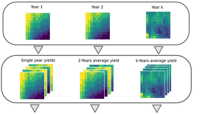
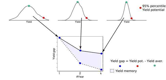
Diagram - Summary of procedure to compute yield gap profiles and yield memory.

Diagram - Summary of procedure to compute yield gap profiles and yield memory.

Figure 1. Summary of procedure to compute yield gap profiles and yield memory. Images from multiple years are averaged to create maps of average yields for varying periods of time. The maps are then used to compute the difference between maximum and average yields for the yield factor domains, and this difference is plotted versus the number of years used in the average (solid line). The dashed line portrays the expected change in yield gap with increasing years if yield patterns were entirely random in space. The shaded area between the lines represents the yield memory.

Within each cluster, a random forest algorithm with weather and soil variables as predictors was used to check the importance of each factor in explaining differences in yield. The importance of each weather and soil variable was computed from permuting the out-of-bag data (data that was not used for building the trees). For each tree, the prediction error of the out-of-bag portion of the data was recorded. Then the same was done after permuting each predictor variable. The difference between the two was then averaged over all trees and normalized by the standard deviation of the differences. The framework presented in Figure 2 summarizes the main steps of all analyses performed in this study.

Diagram - Statistical analysis framework  - crop yield forecasts.

Diagram - Statistical analysis framework  - crop yield forecasts.

Figure 2. Analysis framework showing steps (1) crop yield forecast and data aggregation to 15 km, (2) data summarization (mean and coefficient and variation), (3) spatial constraint clustering, (4) estimate of the stability of the spatial pattern over years, and (5) evaluation of the influence of weather and soil attributes on the stability of spatial patterns.

Results

The cluster analysis with spatial constraint produced 30 yield factor domains for corn and 21 for soybean. Despite the difference in the total number of clusters between the crops, many of the yield factor domains broke out into roughly similar geographical areas. This can be easily visualized for YFD 24 and 16, for YFD 21 and 14, and for YFD 13 and 7, for corn and soybean respectively (Figure 3).

Two important trends were documented among the yield factor domains for both crops:

  1. The higher the yield, the lower the CV of yield over the years and within the same year.
  2. There was a negative correlation between average yield and yield memory. In other words, yield factor domains that had higher yields over the years tended to have a higher variability in spatial pattern from year to year. For example, YFD 24 for corn (comprising northern Iowa and southern Minnesota) had the highest yield among all the yield factor domains and the lowest yield memory, while YFD 14 for soybean (central to north Illinois) had the same behavior. Conversely, YFD 13 for corn and 7 for soybean (mostly within Kansas) had lower yields and higher yield memory.

Another way to estimate the persistence of the spatial pattern across years is to use one year (ranked year) to split the yields from a region into classes, and then to verify if the classes are consistent over the remaining years. For this study, 2017 was used as the ranked year and the yields from this year were divided into deciles. The same division was performed for the remaining years (Figure 4). The significant overlap between the distributions indicates that the relative ranking of yields across pixels tends to vary from one year to the next; however, the more evident positive trend for low-yielding yield factor domains (YFD 13 for corn and 7 for soybean) indicates a higher level of persistence, with high (low) yielding pixels in one year more likely than average to be high (low) in other years. The absence of positive trend and the higher overlap among the distributions for higher-yielding yield factor domains (YFD 21 for corn and 14 for soybean) indicate a lack of persistence for those clusters.

A random forest classification model provided weights for the importance of each weather and soil variable for explaining differences between high and low yield environments. Weather variables generally had greater weights compared to the soil ones (Figure 5). Growing degree units (GDU) was the most important factor splitting the environments in high-yield corn environments and both high- and low-yielding soybean environments. Vapor pressure deficit (VPD) was the second most important weather variable, except in low-yielding corn environments where it was the most important.

The soil variables presented a greater contribution to explaining the yield differences in low-yield environments, for both corn and soybean. This makes sense since those environments had a higher yield memory and soil variables tend to have more consistent effects from year to year compared to weather.

Map - Thematic map with yield factor domains for corn at 15-km resolution, graphs showing the relationship between average corn yield and yield memory.

Map - Thematic map with yield factor domains for soybeans at 15-km resolution, graphs showing the relationship between average soybean yield and yield memory.

Figure 3. Thematic maps with yield factor domains for corn and soybean at 15-km resolution. Color scale representing the yield memory, dark blue means high memory, yellow means low memory. Panels in the right section portraying the relationship between average yield and yield memory, and average yield and coefficient of variation of yield for corn and soybean.

Line and Bar Charts - Yield gap profiles in yield factor domains 13 - low yield - and 21 - high yield - for corn.

Line and Bar Charts - Yield gap profiles in yield factor domains 7 - low yield - and 14 - high yield - for soybean.

Figure 4. Yield gap profiles in yield factor domains 13 (low yield) and 21 (high yield) for corn and 7 (low yield) and 14 (high yield) for soybean. Solid lines represent the decrease in yield gap as the number of years increases for the satellite-estimated yield. Dashed line represents the expected change in yield gap with increasing years if yield patterns were entirely random in space (computed by randomly re-ordering the spatial distribution of yields in each year). The boxplots show the yield distributions for 10 groups pixels, where the groups are defined by the yield deciles in a single year (in this case, the last year of the study period - 2017). The yield distributions are calculated from yields on these fields from nine years prior to the year used to define the groups. Distributions are represented by the median (horizontal line), 25th and 75th percentiles (box), and 10th and 90th percentiles (whiskers).

Bar Chart Series - Mean decrease in accuracy for each variable in yield factor domains 13 - low yield - and 21 - high yield - for corn and 7 - low yield - and 14 - high yield - for soybean.

Figure 5. Mean decrease in accuracy (estimated by removing the variable from the random forest model) for each variable in yield factor domains 13 (low yield) and 21 (high yield) for corn and 7 (low yield) and 14 (high yield) for soybean. Variables are ordered by importance.

Conclusions

Yield memory is a promising concept with potential to help researches to quantity the degree of change in yield spatial patterns over time. It has value as a tool helping to screen environments where factors of interest to researchers are the main drivers leading to differences in yield from one growing season to the next.

Furthermore, in the U.S. this study found a significant negative correlation between corn and soybean yields and yield memory, indicating that regions with higher yields, despite of having more homogeneous yields within a specific growing season, have a lower tendency to maintain spatial patterns from year to year. For high yield memory regions, soil variables had greater weight in explaining yield differences compared to the low yield memory cluster.

Research conducted by Rai A. Schwalbert and Ignacio A. Ciampitti, Kansas State University, as a part of the Pioneer Crop Management Research Awards (CMRA) Program. This program provides funds for agronomic and precision farming studies by university and USDA cooperators throughout North America. The awards extend for up to four years and address crop management information needs of Pioneer agronomists, sales professionals, and customers.

* Data Sources:

  1. Cropland data layer is an annual raster-format land-use maps created by the USDA NASS, based on the Landsat 5 TM, Landsat 7 Enhanced Thematic Mapper (ETM+), the Indian Remote Sensing RESOURCESAT-1 (IRS-P6), Advanced Wide Field Sensors (AwiFS), Landsat TM/ETM+, and AWiFS imagery (the last two since 2010). Since 2008 the raster layers are released on a 30m resolution and cover the continental U.S.
  2. Historical state- and county-level corn yield information is available for downloading from the Internet in tabular form at the USDA/NASS Quick Stats website. This database is released as a point information in a county level (each point is a county/year yield record) without geographical information such as latitude and longitude.
  3. Enhanced vegetation index images were obtained from the MODIS /006/MOD13Q1 collection which provides images with 250-meter resolution (each MOD13Q1 pixel contains the best possible observation during a 16-day period). All the images from this collection were gathered between March 1 and November 10, and between May 1 and November 10, from 2008 to 2017, for corn and soybean respectively, in order to cover the entire growing season for these two crops.
  4. Yearly average temperature and growing degree units (GDU) were derived from the PRISM Daily Spatial Climate Dataset AN81d, this raster layer contains daily and monthly 4 km gridded climate datasets for the U.S., produced by the PRISM Climate Group at Oregon State University.
  5. Vapor pressure deficit was assessed from the Gridded Surface Meteorological dataset that provides a ~4 km daily surface weather raster layers for the contiguous U.S. This dataset blends the high resolution spatial data from PRISM with the high temporal resolution data from the National Land Data Assimilation System (NLDAS).
  6. Soil information (clay, available water content, organic matter content, and pH) was gathered from POLARIS, a map of soil series probabilities that has been produced for the contiguous U.S. at a 30-m spatial resolution and using machine learning algorithms to remap the Soil Survey Geographic (SSURGO) database.


The foregoing is provided for informational use only. Contact your Pioneer sales professional for information and suggestions specific to your operation. Product performance is variable and subject to any number of environmental, disease, and pest pressures. Individual results may vary.

November 2019